Lab 2: Free Fall Lab
Part 1:
In the first part of this lab we found an approximate value of g, and learned how Excel can be used to do repeated calculations with data easily.
Introduction: For this lab, we dropped a mass along an apparatus that generated an electrical shock through the mass and onto a piece of paper 60 times per second, or at 60 Hz. From these marks, we could measure an approximate value for acceleration, and as the only acceleration acting on the mass was gravity, we could approximately find the value for gravity.
Procedure: We started the lab with a demonstration. The professor ran an example of the apparatus in use. Instead of all of the lab groups needing to use the apparatus and waste class time, we used strips of paper from previous labs. We then measured the space in between each mark on the sheet of paper, getting a large enough sample size in order to find a good average. We then plugged all of the data points into Excel, and set up our columns in a way that they would calculate all other data required for our use in the rest of the lab. The lab manual has detailed instructions on how to set Excel up for this experiment.
 |
| Apparatus |
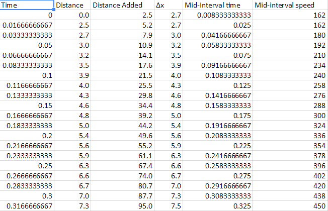
Graphs and Calculations:
All calculations were done by Excel as described by the lab manual.
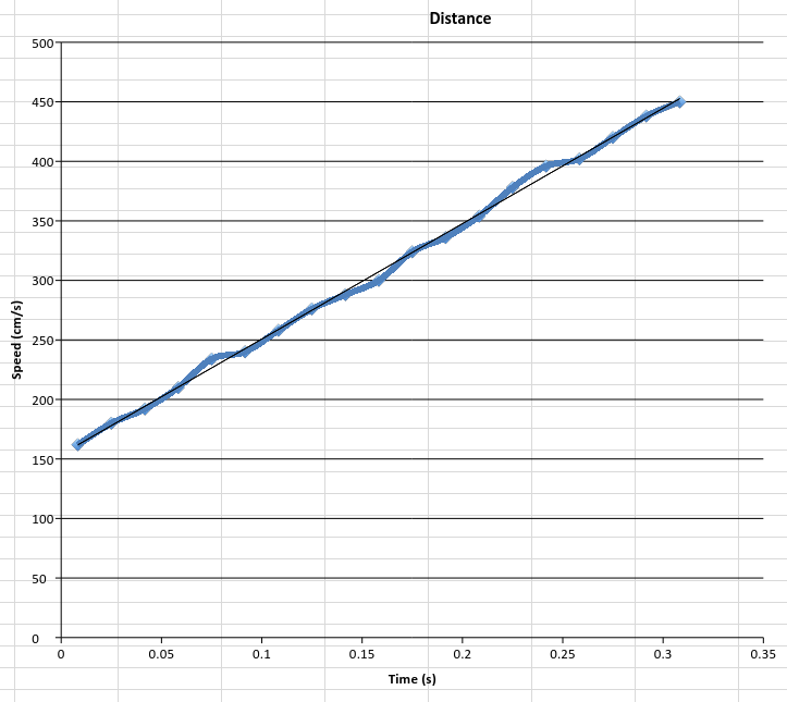
Explanation:
This graph shows the relationship between speed and time for the falling mass. From this graph, we can find the slope of the velocity graph, which is the acceleration. We do this by first finding a linear fit for the data, as no real would data will form a perfect slope, and then finding the slope of that line.
Conclusion/Answers:
The lab provided a relatively accurate approximation for the value of g. After we had calculated the propagated uncertainty of the experiment, we found that the true value of g was within our uncertainty. In order to find a more accurate value of g we would need to use much more complex and expensive equipment.
1.
2. You can get acceleration from the velocity vs time graph by taking the derivative of the line equation, or by finding the slope of the line.
3. The acceleration can be found from the position vs time graph by finding the equation and slope of the line, and then finding the slope of the slope.
There were a few uncertainty in the experiment that would make our value for g not be correct. Air resistance played a small roll, but inconsistencies in the equipment would have been worse. Electrical equipment would possibly not be consistent, causing the dots on the paper to not be exactly 1/60th of a second apart, skewing the experiment.
Part 2:
Data: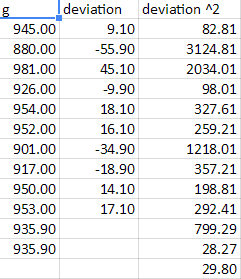
In part 2 of the lab, we used the data for all of the classes values of g and figured out some errors and uncertainty for the value of g. In order to do this we followed the instructions in the lab manual, and used the data in Excel.
Questions Part 2:
1. For the most part, the data across our data was fairly consistent, with only 1 major outlier. The data averaged out to around an incorrect value of g, with only 1 data point getting accurate.
2. The average value of g that was found was lower than the actual value of g. This is due to our equipment not being completely accurate.
3. The classes data did not have a pattern, as they were all different values of deviation from the mean.
4. The systematic errors in our lab were limited to the apparatus, and when measuring the distance of data points on the paper. The apparatus may have not been completely accurate, or may have not been used correctly. When measuring the data points on the strip, the rulers used can only be so accurate, leaving some room for assumption, and therefor errors. Some random errors that may have occurred are the mass catching something when falling, and slowing down, or some fluctuation in the electrical current going to the apparatus that cannot be controlled.
5. The point of this lab was to be an introduction into Excel, and to demonstrate how powerful of a tool it can be when used correctly. It also demonstrated how using Excel can help when trying to understand data. Another point of this lab was to show how data points can deviate from the mean, and how outliers can skew our data. We also learned how to take the average deviation of the mean, and how data falls within a bell curve.
No comments:
Post a Comment