Lab 5 - Trajectories

Lab 5 - Trajectories

Lab Members:

Jarrod Griffin

Christina Vides

Enio Rodriquez

This lab uses our knowledge of projectile motion to predict where a ball will land on an inclined plane from a table.

Introduction:

In this lab we found the initial velocity for a small ball coming off of a table, then used that number to predict where it would fall on an incline. We then ran the experiment and compared our actual and predicted values to find how much they differed.

Apparatus/Procedure:

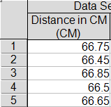
This lab consisted of two different yet similar setups. For the initial set up, we used a pair of V-channels, and set them up as shown above. This created a ramp that we then launched a ball off of. We then found where that ball would approximately land, and placed carbon paper there. We then ran the experiment five times, and then measured the distance from the bottom of the table and created an average distance from these numbers. We then calculated a value for our initial velocity.

For the second setup we used, we kept the ramp the same, and added an inclined plane with carbon paper on it at the edge of the table as pictured. We then did calculations to estimate where the ball would land on the plane. We then ran the experiment and measured how far the ball has fallen down onto the plane, and compared the two values to see how close our calculated value was.

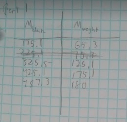
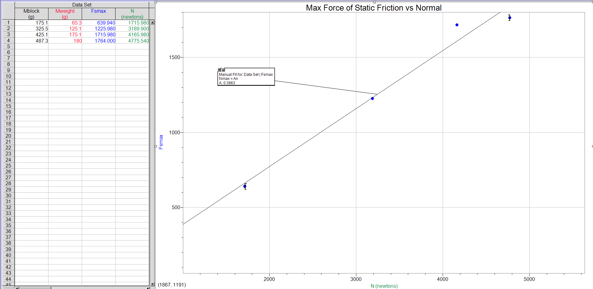
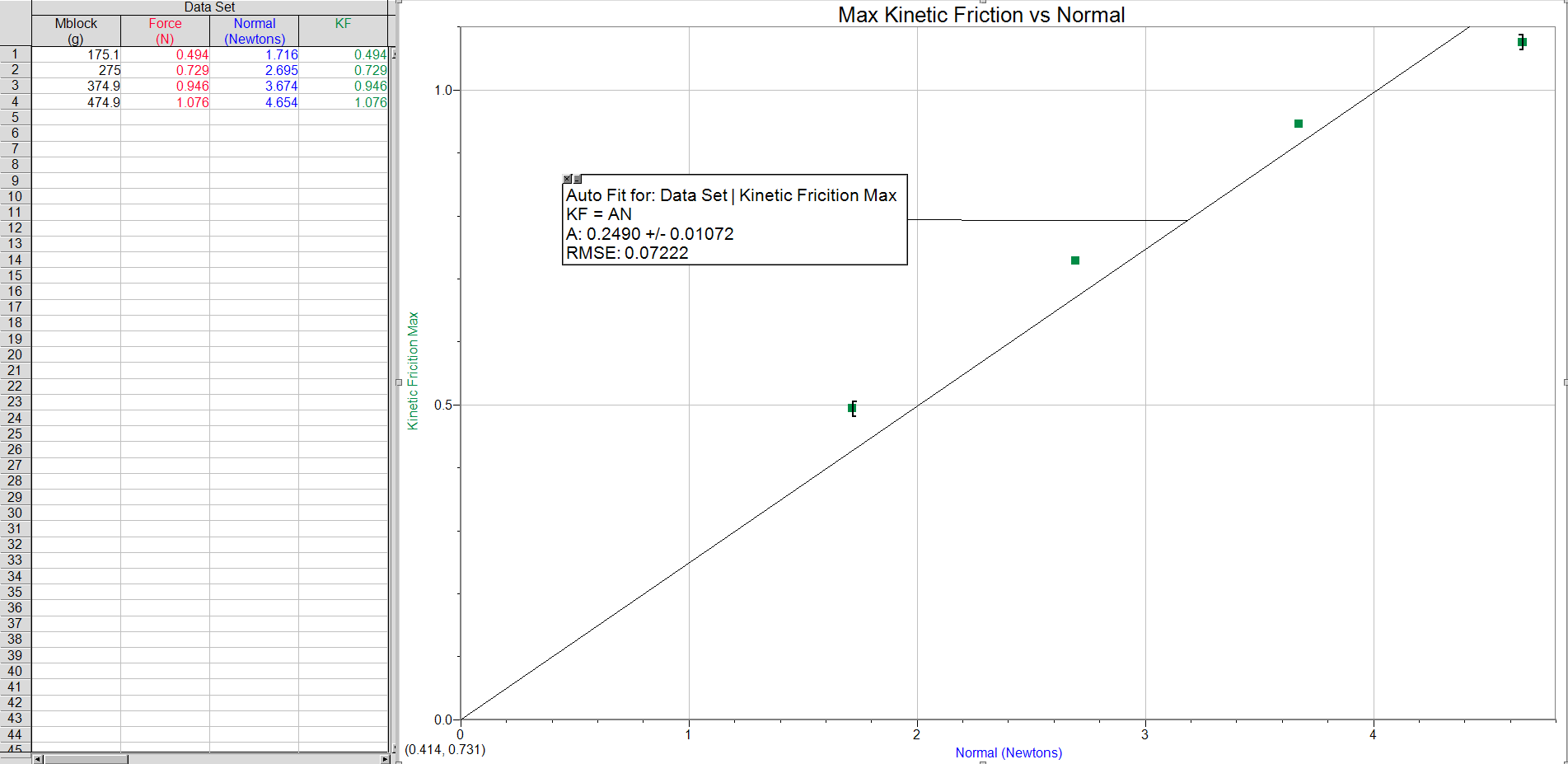
Data:

Calculations/Results:


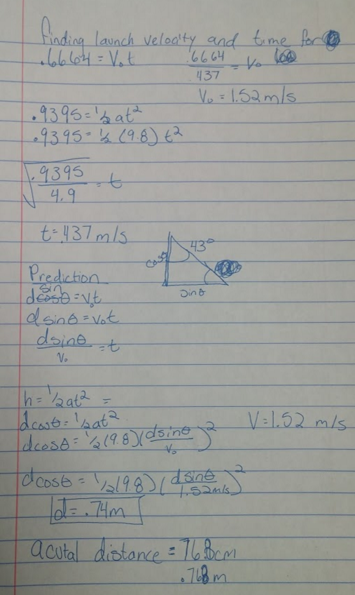
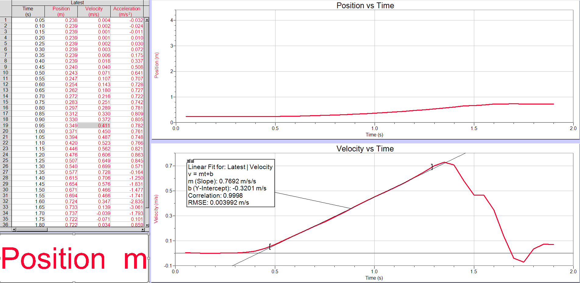
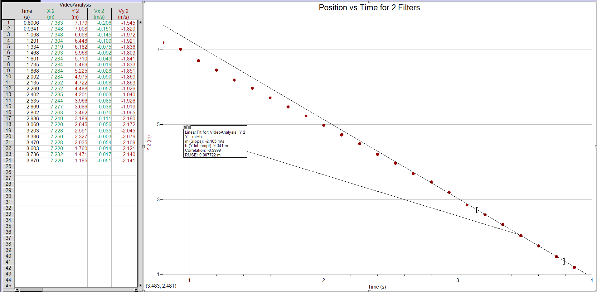
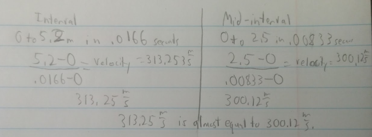
For our initial velocity for our first part, we got the value 1.52m/s. 
We then used that value for part 2 when we calculated where our ball would fall on the slanted piece of wood. For our calculated value of distance we got .74 meters. For our actual value of the distance we received .786m, meaning that our calculated and actual values were very close. 

Conclusion:
Our calculations were very close to what our actual value was. We received only a 5.8% error from the actual and calculated values. We could have had a more accurate calculated value if we took into the fact that friction had played a part during this entire run of the ball. If we used more decimal places, or more accurate measuring devices, our calculated value would be closer to our actual value.

Lab 7 Modeling Friction Forces

Lab 7 Modeling Friction Forces

Lab Members:

Jarrod Griffin

Christina Vides

Enio Rodriquez

This lab helps model kinetic and static friction forces by using a variety off different methods.

Introduction:

In this lab, we used a variety off different setups to measure static friction and kinetic friction. We also used what we had learned about friction forces to estimate the forces, and compare them to their actual values. This lab consisted of 5 different "mini" labs, so the procedures and data will be split into 5 parts.

Apparatus/Procedure

Part 1:

For the first part of the experiment, we used the above apparatus, and continually added mass onto the weight until the block began to move. At that point, we knew that at the mass immediately before it began to move, static friction was at its maximum. Using the mass of both the block and the weight, we could determine a value for the maximum force of static friction. We varied the mass of the block 4 times for this part.

Part 2:

For the second part of the experiment, we used the above apparatus to find a force of kinetic friction on a block. We used a force sensor, that we had calibrated, tied to a block of wood with linoleum flooring on one side, and masses that we changed on top. We varied masses 4 times. We dragged the block with the force sensor, while recording what the force sensor was reading in Logger Pro. We then graphed max kinetic friction vs Normal, and from that slope, received the coefficient of kinetic friction. 

Part 3:

For part 3, we placed the block on a surface, and then raised the surface on one end until the block slid off. We measured the angle that the block had fallen off at using an app on our phones. From this angle, and mass of the block, we could evaluate the static friction force.

Part 4:

For part 4 of the lab, we placed a block on a sloped surface so that it will accelerate once released. We then put a motion sensor on the top of the surface, and recorded the position vs time graph in Logger Pro. We also measured the angle of the board. From these measurements, we could find a coefficient of kinetic friction.

Part 5:

For part 5 of the lab, we set up a system as pictured above, except with a motion sensor tracking the block. We then added a mass to the weight that was heavy enough to accelerate the block. We first estimated what the acceleration would be for the block, then ran the experiment and collected data so that we could find the actual value of acceleration.

Data:

Part 1:

From the above graph, we take the slope to find our coefficient of static friction which for this case, is .3863.

Part 2:

For part 2, we found the force of 4 different blocks. The below graph is an example of 2 of the blocks.

Once we had that data, we then graphed the Max Kinetic Friction vs Normal as shown below. From that, we took the slope and found the coefficient of static kinetic friction.

Part 3:

The angle of the incline for part 3 was 25.4 degrees.

Part 4:

The angle of the incline for part 4 was 20 degrees.

The below graph was created from the data from the motion sensor. The bottom line shows acceleration vs time.

Part 5:

The below graph shows the actual acceleration of our block when attached to a weight. By finding the slope of velocity we found acceleration. Our acceleration was .7692 m/s/s.

Calculations:

Part 1: 

All calculations were done by Logger Pro.

Part 2:

All calculations were done by Logger Pro.

Part 3:

Part 4:

All calculations were done by Logger Pro.

Part 5:

Conclusions:

For this lab, we calculated values for both kinetic and static friction forces. We also found experimental values for both types of friction. The chart under this shows our calculated vs actual values. Our uncertainty was created by logger pro when we plugged in a fit for our data, and other inaccuracies in our equipment. 

Lab 6: Propagated uncertainty in measurements by Jarrod Griffin

Lab 6: Propagated Uncertainty in Measurements

Lab Members:

Jarrod Griffin

Christina Vides

Enio Rodriquez

In this lab, we find the density of metals, and the propagated uncertainty of our measurements.

Introduction:

As the equipment that we use in not 100% accurate, there is always some uncertainty in our measurements. This uncertainty can be amplified when used in equations. This experiment allows us to take measurements, and compare them to actual known values to see how much off we were. We can also compare our propagated uncertainty to how far we were away from the correct value, and check that the actual value lies somewhere within our propagated uncertainty.

Apparatus:

Our equipment for this lab included a caliper, and various cylinders of different metals. We first gathered the measurements for our 2 cylinders, Aluminium and Tin. Our measurements included Mass, Diameter, and Height. We then calculated the volume using the equation for the volume of a cylinder. Once that was completed, we then calculated propagated uncertainty for both Aluminium and Tin, using the square root method of calculation.

Data:

Explanation of Data:

Our experimental value of density of Aluminum was 2.84+-.23 g/cm^3, and 11.31+-2.98 g/cm^3 for Tin.

Actual values of density for Aluminum is 2.7 g/cm^3 and 7.31 g/cm^3 for Tin. Our values for Aluminum were close, and within our uncertainty limits, but for Tin, the measurements were on the very outer limits of our uncertainty.

Conclusions:

This lab was very helpful in learning how propagated uncertainty is calculated and how it can be used to check our values to see if they are remotely correct. In order to get our range of propagated uncertainty smaller, we must use more accurate equipment. While our values of density for Aluminum were very close to being correct, our values for Tin were very wrong. I believe that some measurement was either misinterpreted, or not taken correctly.

Lab 4: Coffee Filters Jarrod Griffin

Lab 4: Modeling the fall of an object with air resistance.

Group Members:                                                                                                                       9/14/2016

Jarrod Griffin

Christina Vides

Enio Rodriquez

In this lab, we developed a model for air resistance by dropping paper coffee filters and measuring their velocity and acceleration.

Introduction: 

For this lab, we used the laptops provided, and their included webcams to take a video of falling coffee filters, with each one varying in weight. We then used the video in Logger Pro to manipulate it and find its position vs time graph. We could then get all necessary data from that graph. 

Apparatus/Procedure:

The equipment need in this lab was a pack of coffee filters, a meter stick, a dark background, a tall ledge, and a laptop with camera. To collect our data we went to a building with a tall ledge from which things could be dropped from. Our professor then set up a meter stick and dark background, then dropped various amounts off coffee filters, from 1 to 6. The meter stick was required to get a distance in Logger Pro, so that it can set the scale for height. We recorded 5 different sets of filters, and then returned to class. In class we then analyzed each video in Logger Pro, to find the different velocities for the different amount of filters. Once we had this data, we calculated the average weight of 1 filter, used a model to find air resistance, and used Excel to find the terminal velocity. We did this so that different amounts of coffee filters could easily be calculated for terminal velocity. We set up Excel as described in the lab manual. 

Part 1 Data:

Here is an example of 1 of the filters dropped and the data points we created. We did this 5 times, once per video. The last few data points were analyzed, and their slope was taken, finding the terminal velocity.

After doing the above for each amount of filters we came up with this data:

The next graph is how we determined our values of k and n. In the graph, A is equal to k, and B is equal to N. For our data, k=.00044+-.00013, and N=1.632+-.21.

We determined the N and k values by using an auto fit for the N v V graph above, and using a power fit.

Part 2 Data:

This is the Excel data that was found after setup, and plugging in the numbers from our part 1 equation. The data is for the weight of 1 filter, and time interval at 1/30 seconds, but can easily be changed to how ever many coffee filters are wanted.

Our model for air resistance worked well but not perfect. Our actual value for V of 1 filter should have been 1.898 m/s.

Conclusions:

This experiment was surprisingly successful and accurate. I incorrectly guessed that the data points would be off by quite a lot and affect the rest of the labs data. Some of the error in the lab could have come from the inaccuracies in the Logger Pro points we inputted, as we can only record at 30 frames per second, and put 1 or less data points every 1.30th of a second. Our equation that we used to model our air resistance was just that, a model. It was never going to be fully accurate in any case.

Lab 3

Lab 3: Non-Constant Acceleration Activity

Lab Members:

Jarrod Griffin

Christina Vides

Enio Rodriquez

In this activity, we work on a problem by hand, and then by using Microsoft Excel. 

Introduction: For this lab, we found an answer for the rocket elephant problem in two different ways, and then compared the accuracy of the answers, and how we could make the answer provided by Excel more accurate.

Apparatus/Procedure: The only material required for this lab was a laptop with Microsoft Excel. We initially worked through the problem, which involved finding how far an elephant would go before stopping, using an analytical approach, and then by using Excel to calculate an answer. When doing the calculations by hand, it required the use of calculus, and hoping that we got an integral that would properly integrate. We followed the procedure of working out the problem by hand that was defined in our lab book. All calculations were already worked out for us in the lab manual. The way Excel was to be set up was also described in detail in the manual.

Excel Data:

Explanation of Data: Once we had "programmed" Excel according to our lab manual, we received the above data. We use Excel to calculate very small values of time, and then use those small values in the rest of the equations. The smaller we get the time interval to be, the more accurate our answer. We use Excel to approximate the value of our definite integral. This would be helpful in case our integral could not be integrated. We determined our value of position by finding when the velocity would switch from positive to negative. At that point, the elephant would have stopped, and began returning along the same path. We also changed our intervals of time into smaller intervals to see how accurate we could get our answer.

Conclusions:

1. When we found the distance analytically, we got the value x=248.7 meters. When we found the value using Excel, we received the approximate value of x=248.63 meters. These two values only differ by 0.03%! If we were to make the time interval smaller, we would eventually reach approximately the same value as we did analytically.

2. In this particular lab we knew when the time interval was small enough when our values of position were almost exactly the same. If we did not know the value of position as we did it analytically, we could find when velocity was equal to zero, giving us the exact position of the elephant. 

3. In order to calculate this easily, we can plug these numbers into our Excel program. 

The position is 154.2 meters.

Excel Data for Question 3:

Lab 2 Wensday September 14th 2016

Lab 2: Free Fall Lab

Part 1:

In the first part of this lab we found an approximate value of g, and learned how Excel can be used to do repeated calculations with data easily. 

Introduction: For this lab, we dropped a mass along an apparatus that generated an electrical shock through the mass and onto a piece of paper 60 times per second, or at 60 Hz. From these marks, we could measure an approximate value for acceleration, and as the only acceleration acting on the mass was gravity, we could approximately find the value for gravity. 

Procedure: We started the lab with a demonstration. The professor ran an example of the apparatus in use. Instead of all of the lab groups needing to use the apparatus and waste class time, we used strips of paper from previous labs. We then measured the space in between each mark on the sheet of paper, getting a large enough sample size in order to find a good average. We then plugged all of the data points into Excel, and set up our columns in a way that they would calculate all other data required for our use in the rest of the lab. The lab manual has detailed instructions on how to set Excel up for this experiment. 

Apparatus

Measured Data: 

Graphs and Calculations:

All calculations were done by Excel as described by the lab manual.

Explanation: 

This graph shows the relationship between speed and time for the falling mass. From this graph, we can find the slope of the velocity graph, which is the acceleration. We do this by first finding a linear fit for the data, as no real would data will form a perfect slope, and then finding the slope of that line.

Conclusion/Answers: 

The lab provided a relatively accurate approximation for the value of g. After we had calculated the propagated uncertainty of the experiment, we found that the true value of g was within our uncertainty. In order to find a more accurate value of g we would need to use much more complex and expensive equipment.

1. 

2. You can get acceleration from the velocity vs time graph by taking the derivative of the line equation, or by finding the slope of the line.

3. The acceleration can be found from the position vs time graph by finding the equation and slope of the line, and then finding the slope of the slope.

There were a few uncertainty in the experiment that would make our value for g not be correct. Air resistance played a small roll, but inconsistencies in the equipment would have been worse. Electrical equipment would possibly not be consistent, causing the dots on the paper to not be exactly 1/60th of a second apart, skewing the experiment.

Part 2:
Data: 
In part 2 of the lab, we used the data for all of the classes values of g and figured out some errors and uncertainty for the value of g. In order to do this we followed the instructions in the lab manual, and used the data in Excel.
Questions Part 2:
1. For the most part, the data across our data was fairly consistent, with only 1 major outlier. The data averaged out to around an incorrect value of g, with only 1 data point getting accurate.

2. The average value of g that was found was lower than the actual value of g. This is due to our equipment not being completely accurate.

3. The classes data did not have a pattern, as they were all different values of deviation from the mean.

4. The systematic errors in our lab were limited to the apparatus, and when measuring the distance of data points on the paper. The apparatus may have not been completely accurate, or may have not been used correctly. When measuring the data points on the strip, the rulers used can only be so accurate, leaving some room for assumption, and therefor errors. Some random errors that may have occurred are the mass catching something when falling, and slowing down, or some fluctuation in the electrical current going to the apparatus that cannot be controlled.

5. The point of this lab was to be an introduction into Excel, and to demonstrate how powerful of a tool it can be when used correctly. It also demonstrated how using Excel can help when trying to understand data. Another point of this lab was to show how data points can deviate from the mean, and how outliers can skew our data. We also learned how to take the average deviation of the mean, and how data falls within a bell curve. 

Lab 1 Monday August 29th 2016

Lab 1: Inertial Pendulum 

In this experiment, we found the periods of known masses, and periods of unknown masses. We then were able to calculate an approximation of the unknown masses from what we had calculated from the known masses. 

Introduction: In the lab, we measured the periods of known masses on an inertial pendulum. From this known mass and period we plotted the data in Logger Pro to create a graph from which we could extract even more data from. It was at this point that we also determined the weight of the pendulum tray, by attempting to get our slope of the line to 1.

Procedure: We started the lab by attaching a inertial pendulum to the table, as shown, and gathered 8 different weights. We then set up a light gate in order to accurately count the periods of time in Logger Pro. We ran the data collection for each weight in order to get a good sample size. Once that was done, we created a data set in logger pro, and plugged in numbers in order to find a number that would make the slope 1, which was impossible, but getting around 1, such as .9999 was acceptable. We then put in two random objects, measured their periods, and calculated their approximate weight. 

Measured Data:

Graph and Calculations:

Period vs Mass of Object and Tray:

Explanation: We graphed the data in order to find a weight of the tray that would be helpful in giving us a slope of 1. Once we were close to this slope of 1, we were able to give a rough calculation of the weight of the two random objects that we had tested.

Conclusion: This lab was very successful. When we calculated the weight of the two unknown objects, and their actual weight, they were, in some cases, very close. Any propagated uncertainty came in the form of inaccuracy of equipment such as scales or light gates, or because the weights were not attatched to the pendulum, and relied only on friction to keep them in place.