Ballistic Pendulum

Ballistic Pendulum

Lab Members:

Jarrod Griffin

Christina Vides

Enio Rodriquez

Joshua Fofrich

This lab uses many different principles, including conservation of energy, and basic kinematics. This lab is to show how all of the about principles can be applied to real world problems.

Introduction:

The goal of this lab is to predict how far a projectile will land from the launcher by first predicting the launch velocity of the projectile, then use kinematic formulas to find a predicted distance. We then launched the ball, and recorded where it fell. We then compared our predicted values of distance to the actual value for distance.

Apparatus/Procedure:

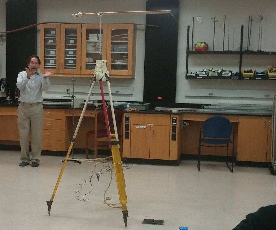
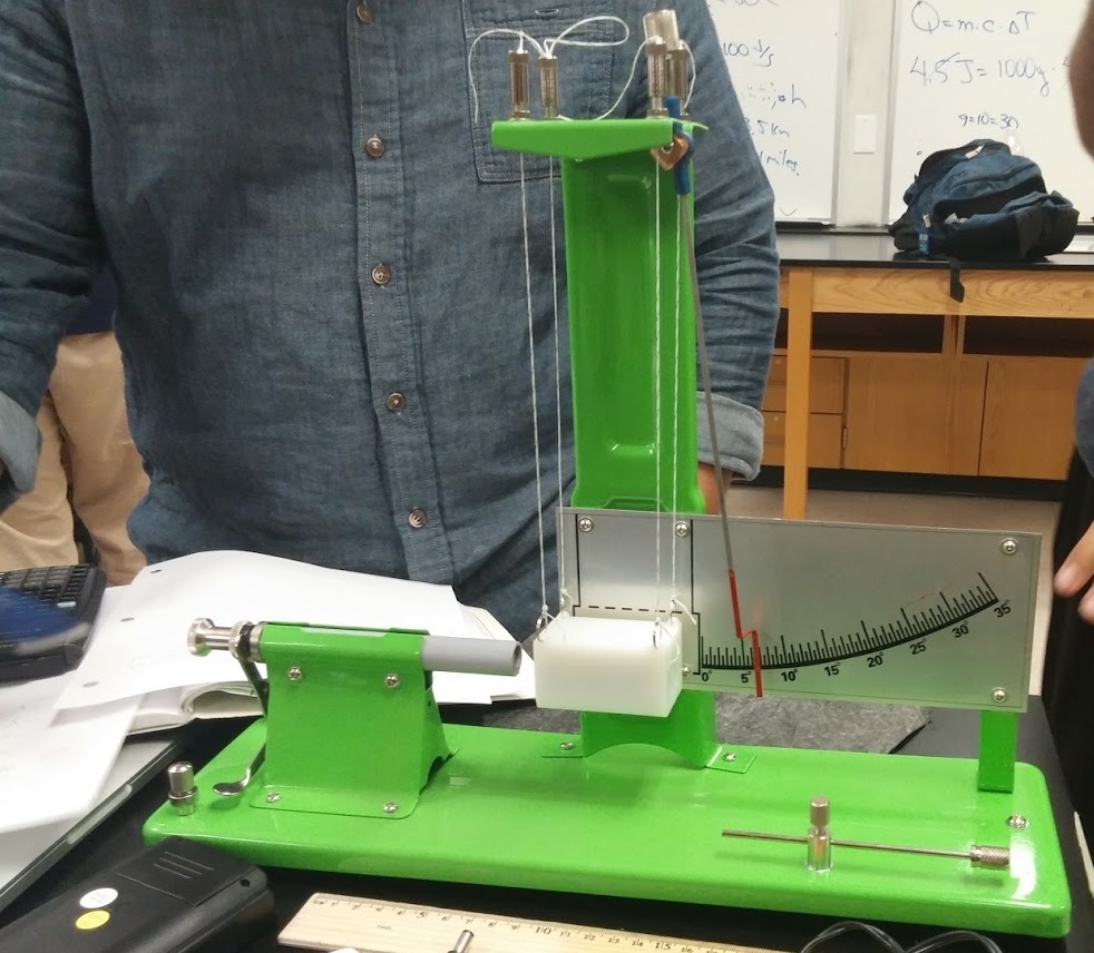
We initially set up the ballistic pendulum so that the launcher would fire directly into the holder, and the projectile would stay in the holder. We then fired this set, and recorded the angle the pendulum reached multiple times to get a good data range. We also weighed all parts of the pendulum and projectile in order to get data for our calculations. Once that was done we used the conservation of energy theorem to find a predicted launch velocity of the projectile. We then calculated where the ball would land in a real world situation. Once those calculations were done, we then launched the projectile onto the floor, moving the pendulum out of the way. We recorded how far the ball went when hitting the ground. Once we had all of this data we could then compare our actual data to calculated data. Below is a picture of our apparatus. 

Data/Calculations: 

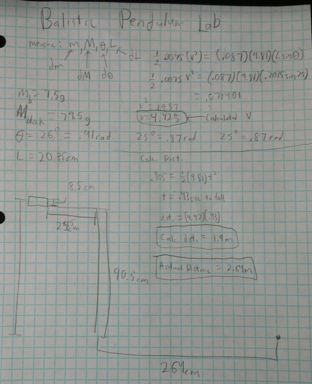
Conclusion:

Our calculations were fairly far off. A large part of this error was in getting our angle for calculating our velocity for the conservation of energy portion of the lab. The data range for our angles was quite large, and will cause a large difference in our velocity, which would affect our calculated distance the projectile went.

Lab 9: Centripetal Force with a Motor

Lab 9: Centripetal Force with a Motor

Lab Members:

Jarrod Griffin

Christina Vides

Enio Rodriquez

In this lab, we use an apparatus to show the relation between angular speed, and the height of the mass at the end of a string connected to the rotating piece.

Introduction:

This lab was a fairly easy one to carry out, mainly because the apparatus was already fabricated and set up correctly. We needed only to change the location of the height measuring device so that the mass would strike it and we could find how height the mass was. The purpose of this lab was to show that as the angular speed increases, the distance of a mass from the ground will also increase.

Apparatus/Procedure:

The apparatus is pictured below. For our procedure, we followed the details in the lab manual. We would first attach a mass to the apparatus, they turn the apparatus on. We then measured the time for 10 revolutions and calculated a period from that data. We then found the height of the mass. The angular speed of the system was then changed. We repeated that process six times to get a large sample set.


Data:



The data above compares the how different our calculated and actual values of w were. A slope of one would mean that they are the same and the calculated were the same as the actual. Our slope of 1.1 means that our values were not that off from each other.

Calculations:





Conclusion:

This lab was done to show the relation between angular speed and the height of a mass. It was also to prove that our calculations can be used in the real world. It was also used to check our calculations against known values and compare how different they are. Our calculations and actual values were very close, with around a 10% error.

Lab 12: Conservation of Energy in a Mass

Lab 12: Conservation of Energy in a Mass-Spring System

Lab Members:

Jarrod Griffin

Christina Vides

Enio Rodriquez

In this lab, we  predict how Kinetic Energy, Gravitational and Elastic Potential energy will appear on a graph vs time, and then compare that to actual values we get from doing the experiment. We also check to see if the total energy of the system stays constant.

Introduction:

For this lab, we used a Mass-Spring System to prove that the conservation of energy theorem is true, and can be applied in real life events. Will also used this lab as a chance to test what we know about the above energies. 

Apparatus/Procedure:

We set up our lab in accordance with the lab manual. We first measured the length and weighed the spring, and verified the weight of our mass. We then zeroed and reversed the distance sensors. We accomplished this by referring to the lab manual. We used a laptop and Logger Pro to record data. We changed the software, as described in the lab manual. The procedure for how each graph was made will be written below each graph in the data section of this write up. Below is a picture of our setup. 

Graphs/Data:

My Predictions:

In order to find the above calculations, we created different columns for each energy, and used the formulas shown below to have Logger Pro calculate the data required for each energy. 

These graphs show where the energy in the system is going at different times and different positions. The blue time, total energy in the system, should stay constant in a perfect world, but as shown in the graph above it does not. It looses small amounts of energy due to outside sources. Our calculations were also not perfect, as the spring will not be perfectly constant throughout its stretch as they were not perfect springs. 

Conclusion:

Only some of my predictions were shown as correct. Our data for this lab was actually very nice, and helped us in analyzing the data. This lab was very interesting, and having a visual representation of different energies helped me to understand them more. Each graph makes since, even if they are a bit off. In order to check if they make sense, we looked the the formulas of how each was calculated and plugged different points of data in for each, just to make sure they were close to correct.

Lab 15: Collisions in Two Dimensions

Lab 15: Collisions in Two Dimensions

Lab Members:

Jarrod Griffin

Christina Vides

Enio Rodriquez

The purpose of this lab is to check if kinetic energy and momentum are conserved in a two dimensional collision.

Introduction:

In this lab we used a glass table, two small balls, a computer and our smartphone cameras in order to complete this experiment. We used our smartphone cameras on a slow motion setting in order to get a video file we can analyze in Logger Pro and get precise position measurements for each ball. From these position measurements, we can find the velocity of the balls before and after the collision.

Apparatus/Procedure: 

We set up our lab as described in the lab manual, except instead of using a camera that connects to our laptops, we used the cameras on our smart phones that can record at a higher frame rate, giving us more frames per second to collect data from. We wanted this so that we could get more precise data, giving us more real world results. Once we collected our data and analyzed it in Logger Pro, we used linear fits before and after the collision in order to give us velocities for both balls before and after collision. A sample of the apparatus is pictured below. 

In order to check to see if kinetic energy and momentum were conserved, we found the velocity as mentioned above, and plugged them into our two equations for conservation of energy and momentum.  We repeated this experiment two times with two different types of balls, metal, and clear/glass.

After Collision between Glass and Steel:


Before Collision between Glass and Steel:

Data/Calculations:

Steel Ball vs Glass Ball:

This is a sample calculation done. I did this type of calculation for the other set of balls that collided. For the above calculations, I used the conservation of energy equation in order to verify if the energy was conserved, which it was not. I also used the conservation of momentum equation to check if it was, which it was.

We calculated the velocity of the center of mass by using a linear fit in Logger Pro. We found the position on the center of mass by using a feature built into Logger Pro that plotted the position of center of mass if given the masses of the two objects.

Graphs:

Conclusion:

In this lab, we showed that momentum was in fact conserved, while kinetic energy was not. We lost kinetic energy due to small amounts of heat, friction, and sound. We proved this by finding the velocities of both balls before and after impacts, and by then using the conservation of momentum and kinetic energy theorems to verify if the energy and momentum were actually conserved. We had predicted that momentum would be conserved, but that energy would not be, which we proved to be true.

Lab 11: Work-Kinetic Energy Theorem Activity

  Lab 11: Work-Kinetic Energy Theorem Activity

Lab Members:

Jarrod Griffin

Christina Vides

Enio Rodriquez

In this lab we will use the Work-Kinetic Energy Theorem to show that the area under a force curve will be equal to the Kinetic Energy at that point.

Introduction:

In this lab we used a motion and force sensor along with a cart and spring to show the relationship between Work and Kinetic Energy. Once we received a nice Force v Position graph, we calculated the kinetic energy, and compared the two graphs side by side, and then proved our theory by taking the area under the Force v Position graph. 

Apparatus/Procedure:

We set up our apparatus as described in the lab manual, with a cart attached to a spring, and placed on a cart track with a motion sensor and force sensor attached. This set up is shown below. Our setup did not change between the two experiments. 

Once we set up our experiment we followed the procedure outlined in the lab manual. We first calibrated our force and motion sensors. We then opened the Logger Pro file on our computers. We then ran an experiment where we moved the cart closer to the motion sensor in order to get a force v position graph. For our second experiment, we stretched the spring and cart system some distance away from the resting point. We recorded the data in Logger Pro and created a calculated Kinetic Energy column.

Data/Graphs:

Conclusions:

The work done on the cart by the spring should be equal to the maximum kinetic energy in the cart. Our data above shows that this is true. While not equaling perfectly, they are very close for this experiment.

Work is equal to the force times the distance. Work is also equal to the change in kinetic energy. If we find the change in kinetic energy, that value should be equal to the area under the curve up until that point. This is proven by taking the integral of the first graph and comparing it to the maximum value of the second graph.

Lab 13: Magnetic Potential Energy

Lab 13: Magnetic Potential Energy

Lab Members:

Jarrod Griffin

Christina Vides

Alex Reyes

This lab will help us model the force of Magnetic Potential Energy.

Introduction:
In this lab, we use an air-track glider and two magnets to prove that the conservation of energy theorem still applies to Magnetic Potential Energy. We accomplished this by doing this lab in 2 parts as will be discussed in the next section.

Apparatus/Procedure:
For the first part of this lab, we set up an air track on an angled surface, measured the angle the track was at, and then turned the track on with the cart so that the cart would more towards the magnet. Once it arrived at the magnet we allowed the cart to settle, and then we measured how far the cart was away from the other magnet. We then repeated this with different angles 6 times. Once this was done, we then found the magnetic force that was applied to the cart. Then we graphed the force vs the separation distance. From that graph, we could use Logger Pro's power fit option and received an equation U(r) for the interaction between the magnets. Our measurements were within .01 mm from the calipers, and in Logger Pro, A's uncertainty in the equation was +-2.322e-05, and B's was +-0.06026. Once that was done, we then set up the second part of the lab. In the second part we placed the track and cart on a level surface, and placed a motion sensor at the end of the track, but far enough away that the motion sensor will still be able to 'see' the cart at all times. We then pushed the cart along the track and recorded the data of the carts position. We then determined the relationship between the distance the motion detector reads and the separation distance between the magnets, as described in the lab manual.


Measured Data:

For our separation distance, we measured .33 meters.


Calculated Data:






Conclusion:

This lab turned out well, with only a few bad points of data that were causing us issues. In the Force vs Separation graph, once the first two data points were taken away, our power fit was excellent. In our Energy vs Time graph, we had an issue of a small blip in our position data, creating the bad looking graph shown above. We also had an issue when determining our separation distance.