Lab 21: Mass-Spring Oscillations Lab

Lab 21: Mass-Spring Oscillations Lab

Date Completed: November 23rd 2016

Lab Members:
Jarrod Griffin
Christina Vides

Enio Rodriquez

Introduction:

In this lab, we worked as a team of smaller groups, each with one spring. We found spring constants and masses, then found the period of the spring with various masses, then compared our data with the class. This lab used our knowledge of springs and periods to calculate various data points.

Procedure/Apparatus:

We initially were assigned one spring. We measured the weight of the spring and then used the effective mass formula provided in the lab manual to calculate the effective mass of the spring. One we determined that, we found the spring constant by measuring the length of spring before mass was applied, and then after mass was applied. We used those values in the F=kx formula. Once that constant was found we found the oscillation periods for 5 various masses and recorded them. We then plugged the data into Logger Pro to analyze. Below is a picture of our apparatus that we set up as described in the lab manual.

Measured Data:

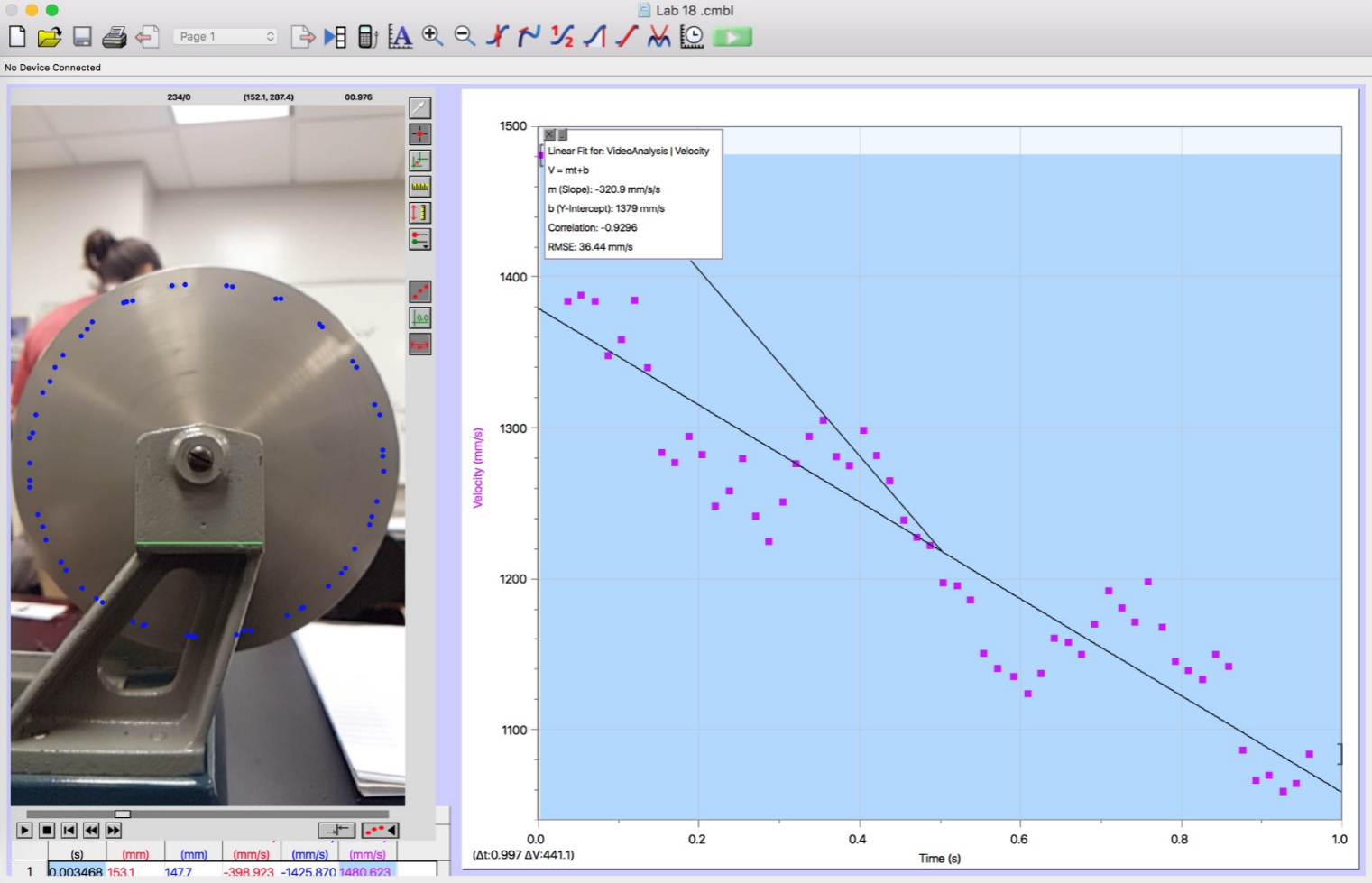
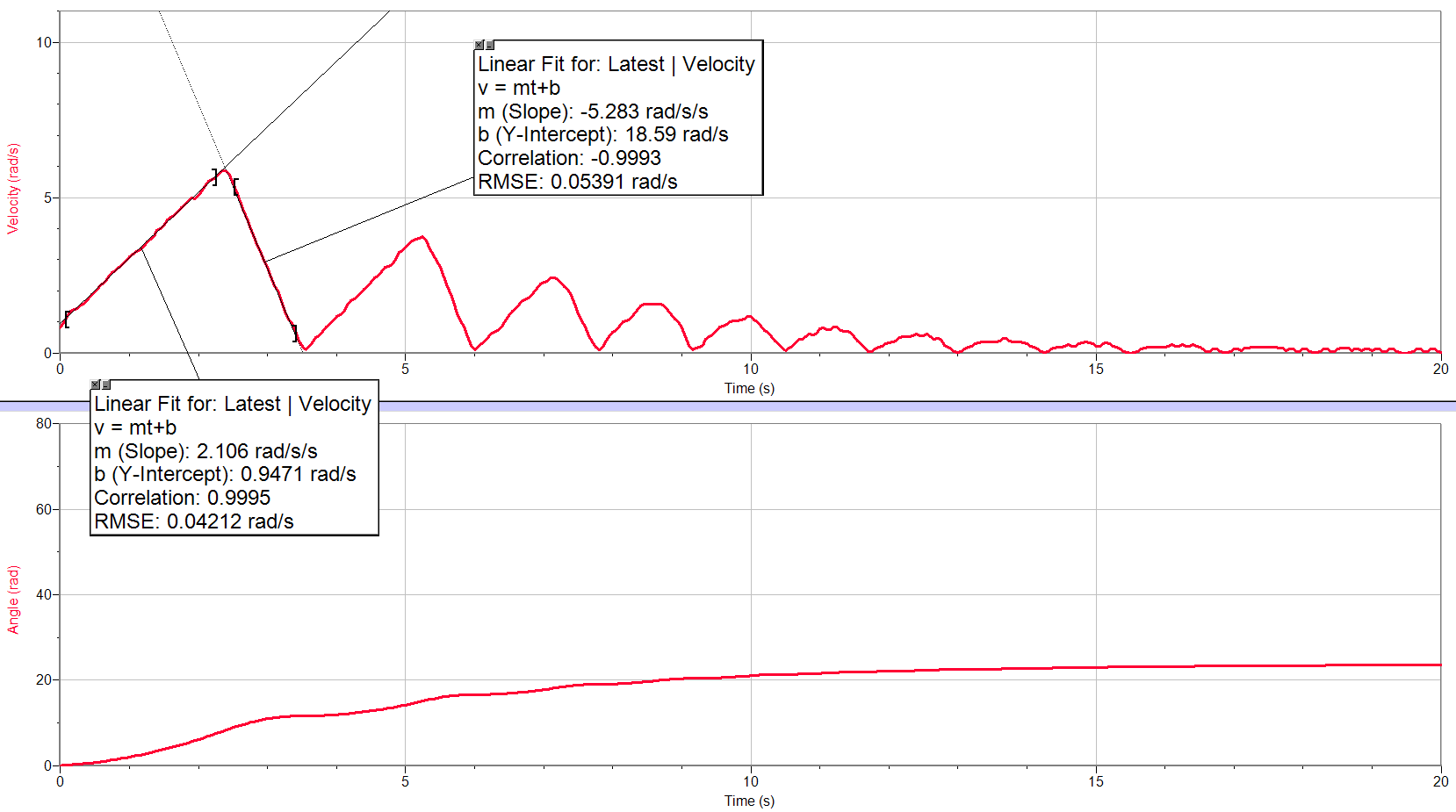
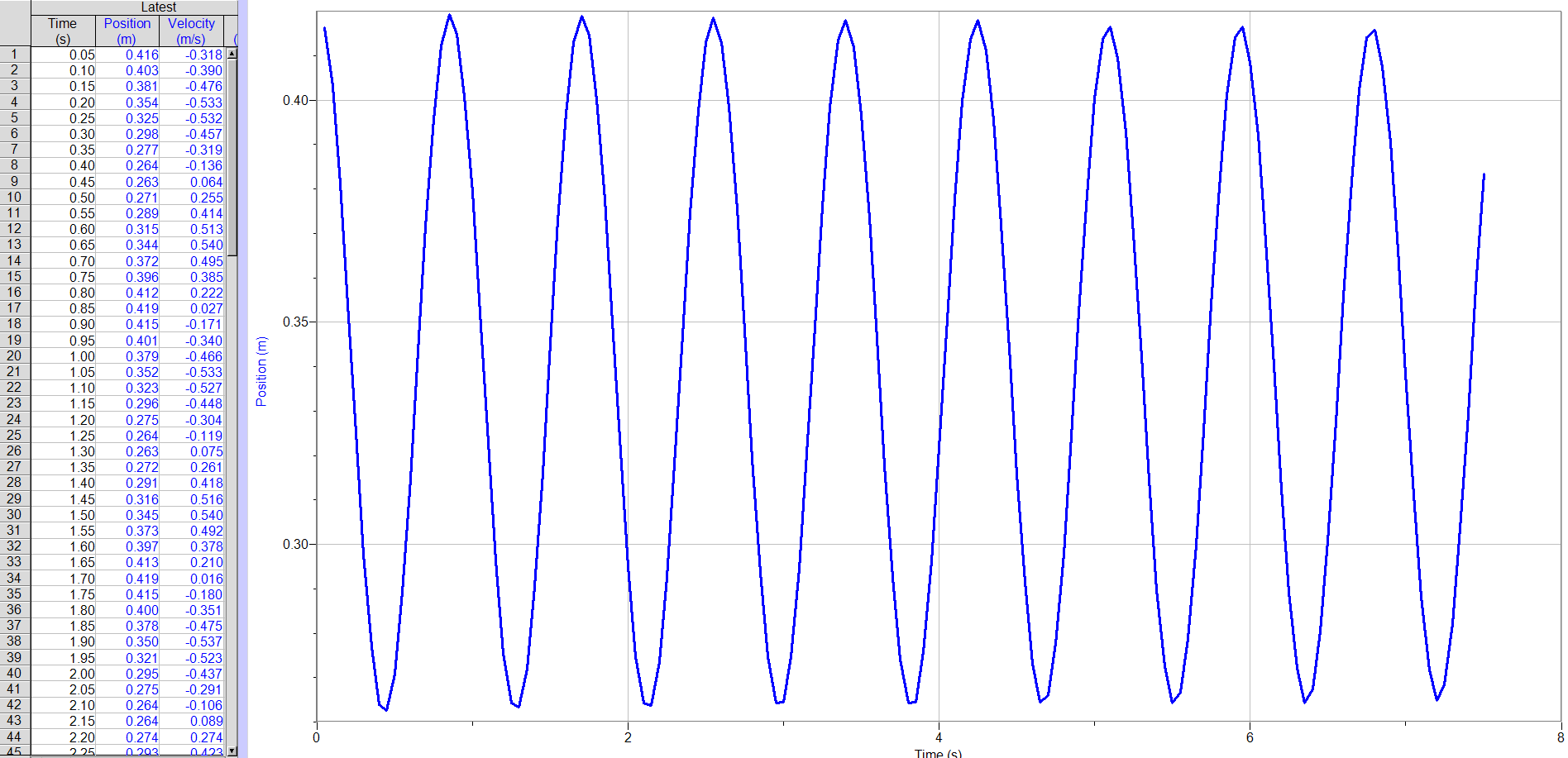
We measured the period of the spring with various masses by using Logger Pro. We could find the time between two peaks of the position, then measure out 10 of them and take an average of the time between two peaks. Below is an example of the Logger Pro graph we used.

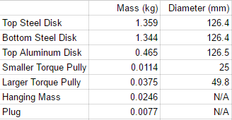
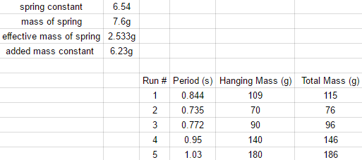
We also took measurements of various masses, included in the spreadsheet are our period data points.

We also collaborated with the class in order to get spring constants and masses for the other springs.

Calculated Data:

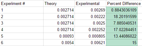
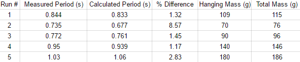
In order to calculate our theoretical values for period of the spring and different masses we used the equation 2𝜋√(m/k)=T.

Below is our graph of Period vs Hanging Mass. We checked to see if our data was accurate by using a curve fit and checking how well our data lined up. We used the T=Ax^0.5 power fit as shown below.

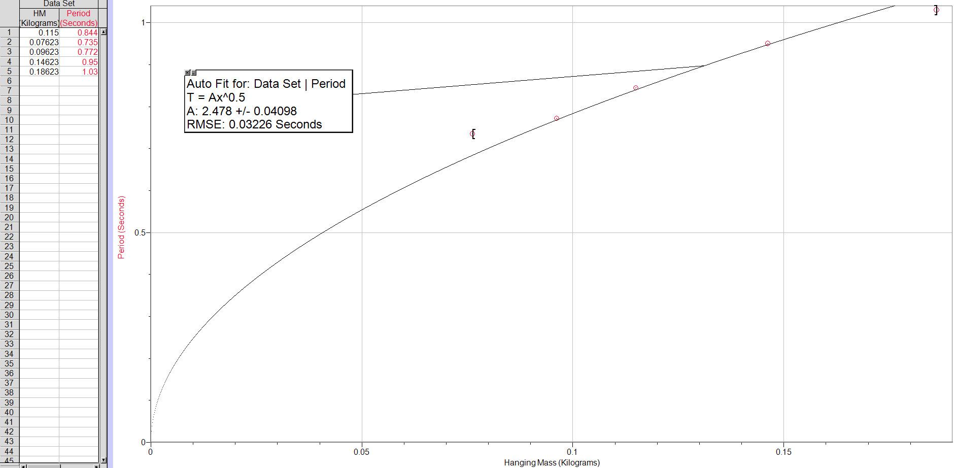
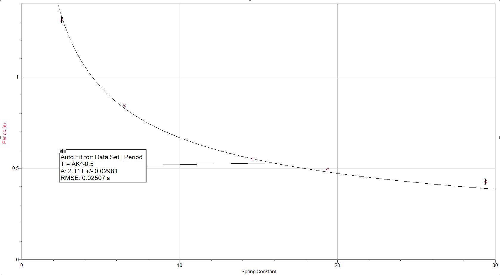
Our data fit very well, except for one data point. We then graphed the class periods vs their spring constant values. We used the same curve fit function for that data as shown below and discovered it fit well, just like our other graph with no majorly different data points.

Conclusion:

Our percent errors were very small for this lab. Springs and oscillations work well as there is little friction and other outside forces working on it. One issue is that not all springs are perfect, although ours were very close. 

5. If our k value was off by 5%, if would effect the period calculations by around 3.5%. 

6. If the spring constant would increase, the spring would become stiffer, and also requires more force to stretch the spring. The spring will be slow to stretch with the same amount of mass as before. The spring force will be stronger, meaning a weaker effective downward acceleration from gravity, and slowing the mass, therefor slowing the period.

7. If the mass of the system increases, then so does the force due to gravity. More mass also means more stretch in the spring, meaning that the spring force will also increase. When both forces increase, the acceleration down and up will increase, reducing the time to complete a cycle up and down and up, making the period smaller.

Lab 20: Conservation of Linear and Angular Momentum

Lab 20: Conservation of Linear and Angular Momentum

Date Completed: November 21st 2016

Lab Members:
Jarrod Griffin
Christina Vides
Enio Rodriquez

Introduction:

In this experiment we investigate conservation of different momentums. In order to do this we rolled a ball onto a moment arm that was on a freely rotating disk. This lab was done as a class, so almost all data will be the same between students. 

Procedure/Apparatus: 

We started this lab by first measuring almost all aspects of the experiment, including heights, masses, and radii. We then set up the ramp ball system on the edge of a table, and found its velocity as it left the ramp. We then placed the ramp so that it would hit the moment arm of the disk and the ball would stick, transferring all of its linear momentum into rotational momentum. We recorded the rotations of the disk. We then calculated our data and made a prediction of what our experimental values would be. 

Measured Data:

We found alpha by taking the average alpha from graphs in Logger Pro that are pictured below.

Calculated Data:

We used the conservation of momentum theorems to derive an expression where the only unknown variable was W. This allowed us to calculate what W would be in a perfect world. We can then compare this to actual data we have. 

Conclusion:

This lab was very successful. Our percent errors were both below 5%, meaning that our setup was very good with very little outside involvement such as friction and other resisting forces. This lab showed us that the conservation of momentum theorems hold true even in the real world where outside forces act upon the system. Some uncertainties in the system are all measurements we took. We took almost all measurements with a meter stick, something that can only be so accurate.

Lab 19 Conservation of Energy and Angular Momentum

Lab 19 Conservation of Energy and Angular Momentum

Data Completed: 11/21/2016

Lab Members:
Jarrod Griffin
Christina Vides
Enio Rodriquez

This lab attempts to show a real world example of conservation of angular momentum and conservation of energy, and when to use the two in a real world experiment.

Procedure/Setup:

In this lab we set a pendulum up so that it will strike a ball of clay on the ground. We then used video capture along side Logger Pro to get the height the meter stick and clay combination rose to. In order to calculate an estimated height for the meter stick and clay, we had three main steps that will be listed in calculations.  A picture of this setup is shown below. 

Measured Data:

We found the height that the meter stick and clay had risen to by using Logger Pro and a video of the swinging apparatus. We found its maximum vertical position after swinging through its equilibrium point, and then found that point on the X/Y plane we placed in Logger, along with setting the scale. This will give us a close value for maximum height of the end of the meter stick. 

Maximum height reached by end of meter stick(0.1323m):

Calculated Data:

To calculate our data, we followed a basic three steps. We first found the rotational velocity as it swung through equilibrium and right before it hit the clay, second, we then applied conservation of rotational momentum for during the collision, and lastly applied conservation of energy after the collision. We could not apply conservation of energy to the entire problem as there was energy loss due to the deformation of the clay in the impact. We must also take into account the change in center of mass of the system after collision.

Conclusion:

With a small percent error of about 5%, this lab was a success. Some of the percent error is explained by friction from the pivot, and from the clay scraping along the ground, even though we used a paperclip to eliminate much of that friction. Even more of the error can be explained from the measurements of our data, within Logger Pro, and the measurement of the length of the meter stick from the pivot. 

Lab 17: Moment of Inertia of a Uniform Triangle

Lab 17: Moment of Inertia of a Uniform Triangle

In this lab, we determined the moment of inertia of a right triangle in two different orientations and then compared them. 

Introduction:

This lab gives us a visual and numerical representation of different moments of inertia of the same object that is just in different orientations. We used the same setup as in the Rotational Acceleration Lab to measure values for angular acceleration α. 

Apparatus/Procedure:

For this lab, we used the exact same setup as in lab 16, with the only difference being that we placed a triangle on top of the top rotating disk in two different orientations. 

We took data from this apparatus by using Logger Pro, just as we did in the previous lab. We ran 3 experiments. Initially we ran one without the triangle on it, then one with the height of the triangle as large, then one more with the height as small. 

Data/Calculations:

Actual Values:

Theoretical Values:

Conclusion:

This lab, just as with the other moment of inertia lab, went terribly. I believe that one or more of our measurements was very wrong, or our calculations were using the incorrect data. We can account some percent error for friction in the system, but not enough to get an 85% difference in some data. 

Lab 18: Moment of Inertia and Frictional Torque

Lab 18: Moment of Inertia and Frictional Torque

Introduction:

In this lab, we find the moment of inertia of a rotating non uniform disk, and then also find the frictional torque on its axles. Once we have this information, we could then predict how long it would take a cart to slide down an angled track. 

Apparatus/Procedure:

For this lab, we used a large pulley, a cart, a track, and various calipers. We followed the procedure described in the lab manual and took almost every measurement we could. We then calculated the moment of inertia of the pulley by adding the moments of inertia of each individual piece. Once we had this information, we then calculated our frictional torque by taking a slow motion video of the pulley slowing down and then analyzed it in Logger Pro. We took the slope of the velocity to find the angular deceleration α. These calculations and graphs are all located below. Once we found that, we could then estimate the time a 500 gram cart on a 40 degree incline would take to travel a meter. We then found the actual time it took and compared the two. 

Data/Calculations:

Calculating total inertia.

Graph used to find angular deceleration.

Calculating frictional torque.

Predicting time the cart will take to travel 1 meter at 40 degrees. The cart weighs 500 grams. 

Conclusion:

With a error of only 0.67% our experiment was a great success. Even with the relative inaccuracies of our measurements our time was very close to actual values. 

Lab 16: Angular Acceleration

Lab 16: Angular Acceleration

Lab Members:

Jarrod Griffin

Christina Vides

Enio Rodriquez

Part 1:

In this lab, we are introduced to the physical concepts between angular kinematics.

Intro:

 This lab provides a real world representation of many variables in angular kinematics. We used an apparatus that is described below in order to accomplish this. We also used Logger Pro to allow us to collect and get a visual representation of the concepts. 

Apparatus/Procedure:

For this lab, we used an apparatus that involved two spinning disk that uses compressed air in order to essentially eliminate friction. We used various different setups of this apparatus to get different results from the lab. The various types of setups are described in the lab. We measured the weight and radius of all components of the apparatus and recorded the data. 

In order to take data, we attached a mass to one end of the string and attached the other end to the center of the torque pulley. This setup was varied multiple times.

Data/Calculations:

We found the above data values by using Logger Pro. We took linear fits of the data for when the mass was moving up and down. We then averaged them in order to more easily work with the data and to compare it. Below is an example of the graph of data we got using Logger Pro. We repeated this test with varied parameters 6 times.

Conclusion:

Part 2:

In part 2 of this lab, we used formulas provided in the lab manual, and our collected data to compare our values for known values. Below is a sample calculation for how we calculated the data. Below that will be the results of all data.

Our results were not the best for this lab. I believe that the errors in the experiment were due to unknown friction in the rotating pulley that guided the string, and other frictional forces. We also had uncertainty in each of our measurements, as we had measured almost every part of this apparatus. Overall the experiment went well, but only one data point came close to what we had expected in our theoretical values.